How Certain Is a Cyber Risk Quantification Result?

On this page
A cyber risk quantification (CRQ) result arrives as a range: a most likely loss, a band of probable losses, and a tail of rare but severe ones. This article is about cyber risk quantification uncertainty: where it comes from and how to read it.
Modern CRQ, including FAIR-based analysis, is a simulation. It uses Monte Carlo methods to play out thousands of possible years, using estimates of how often loss happens (frequency) and how much it costs (magnitude, or severity).[1][2] The spread of those simulated years is the model being honest about what it knows and what it does not.
This article shows you how to read that honesty. You will learn the two kinds of uncertainty in every result, how to spot each one, how to tell frequent losses from rare catastrophic ones, and what makes a result more certain over time.
Two kinds of uncertainty
Risk scientists separate uncertainty into two kinds.[3] The difference matters, because only one of them can be reduced.
1. Randomness in the world. Some events are rare by nature. Even with perfect knowledge, no one can say which year a severe attack will land. A fair die is a good example: you know everything about it, and you still cannot predict the next roll. Scientists call this aleatory uncertainty. More data does not remove it. A good result shows it plainly.
2. Gaps in what we know. When the model lacks facts about your organization, it fills them with estimates. How strong are your controls? How is your network built? What does an hour of downtime cost at each site? Each estimate widens the range. Scientists call this epistemic uncertainty. This is the part better data reduces.
| Randomness in the world | Gaps in what we know | |
|---|---|---|
| Where it comes from | The rare, unpredictable timing of events | Missing facts about the environment |
| Example | A once-in-decades attack could land next year or in 30 years | Control strength estimated from industry averages instead of your own evidence |
| Does more data reduce it? | No | Yes |
| What a good result does | Shows it as a long tail | Narrows it as evidence replaces assumptions |
Most CRQ results contain both. When a result looks wide, the useful question is: how much of that width is the world, and how much is us?
How to read uncertainty in a result
You do not need to be a statistician to judge how certain a result is. Look for five signals.
| What to look for | What it tells you |
|---|---|
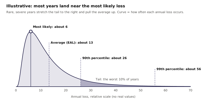
| Width of the probable band. Compare the low end and high end of the middle range, such as the 10th to 90th percentile. | A band where the high end is many times the low end means the inputs are uncertain. A tighter band means the inputs are better known. |
| Average versus most likely. Compare the average, called the expected annual loss (EAL), with the most likely annual loss. | If the average sits far above the most likely value, a few severe outcomes are pulling it up. That is a long tail. |
| Frequency below one. Check the expected number of loss events per year. | A value of 0.1 means about once in ten years. Most years show no loss at all, so judge the scenario by its severity and its tail. |
| The tail. Look at the worst outcomes, such as the 95th or 99th percentile. | This shows how bad a bad year could be. It matters most for insurance limits, capital and board risk appetite. |
| What drives the spread. Look for a sensitivity view that ranks inputs by how much they move the result. | The inputs at the top are where better data would narrow the range most. |
The last signal is the most useful for planning. It turns "the result is uncertain" into "the result is uncertain because of these three inputs." That tells you exactly where better information pays off.[2]
Many CRQ reports also show a loss exceedance curve: the chance that losses will exceed any given amount in a year. Our article on how to read a loss exceedance curve explains it in detail.
Frequent losses versus rare, severe losses
Every loss scenario sits somewhere between two extremes. Some losses are frequent and small. Others are rare and severe. They call for different decisions, and they look different in the results.
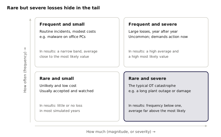
Frequent, smaller losses show up in most simulated years. Their band is fairly narrow, and the average sits close to the most likely value. You can budget for them, much like any other operating cost.
Rare, high-magnitude losses show up in only a few simulated years. In most years nothing happens, so the most likely annual loss can be zero or close to it. The few severe years pull the average up and stretch the tail. Read only the most likely value and the risk seems to vanish. Read the tail and it is often the largest exposure in the business.
Two rules of thumb help:
- If the expected frequency is well below one per year, judge the scenario by its magnitude and its tail.
- If the average is many times the most likely value, a rare, severe outcome is driving it. Ask what that outcome is and whether you could survive it.
Rare and severe is the pattern most industrial (OT) risk follows. A long plant outage, damaged equipment or a safety incident may happen once in decades, yet cost more than years of routine incidents combined. Market-wide estimates show the same shape: OT cyber risk carries roughly $31.1 billion in annual financial risk, and up to $329.5 billion in a severe, 1-in-250-year event.[4]
Why OT results start wider
Industrial (OT) cyber risk is hard to measure for a simple reason: the events that matter most are rare, and few are made public.
- Public evidence is thin. Serious attacks on plants, pipelines and grids are uncommon. When they happen, owners often share little about the cost (beyond what is mandated by public disclosure regulation).
- Actuarial data is limited. Insurers have far less claims history for cyber-physical loss than for data breaches. There is no long record to fit a curve to.
- Every site is different. Two plants in the same industry can have very different networks, controls, equipment and cost of downtime. Industry averages hide those differences.
Waiting for decades of loss history is not an option. Simulation is the practical way to understand rare but catastrophic losses. It combines what is known about threats, controls and costs, and plays out the range of possible years.
The trade-off is that a simulation is only as specific as its inputs. When it runs on public information and industry estimates, the ranges must stay wide to remain honest. That width is mostly the second kind of uncertainty: gaps in what we know about your environment. Which brings us to the good news.
What reduces uncertainty: better data about your environment
The first kind of uncertainty, randomness, stays. The second kind, gaps in knowledge, shrinks each time an assumption is replaced with evidence from your own environment. Analysts call this the value of information: data is worth collecting when it narrows a range that affects a decision.[2]
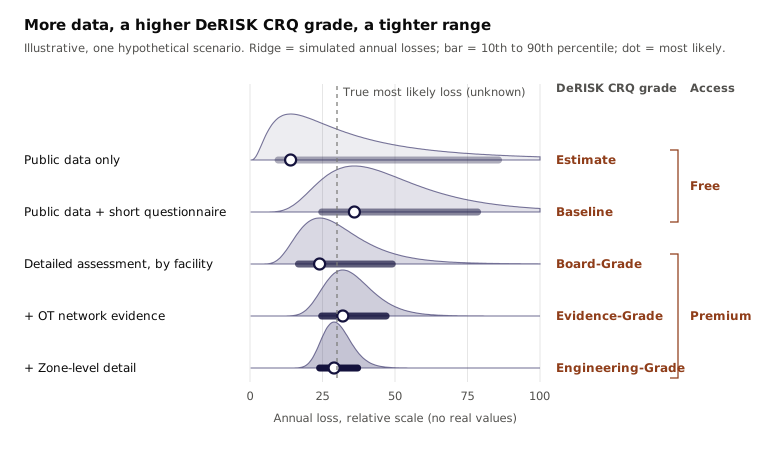
In practice, data tends to arrive in steps or a journey. Each step describes the real environment more closely:
- Public data only. Company size, industry and public records. The model fills everything else with industry estimates. Ranges are wide.
- Public data plus a short questionnaire. A few key facts about the organization replace the most important assumptions.
- A detailed assessment, facility by facility. Controls, practices and the cost of downtime for each site. Results begin to reflect how each site actually operates.
- OT network evidence. Data from the plant network itself, such as firewall rules, network diagrams and monitoring data. This evidence checks and adds to the self-reported answers.
- Zone-level detail. The same evidence resolved to the network zones inside each site, so the model sees which critical systems are exposed and how.
The chart above is hypothetical and shows the pattern only. Two things change as data improves. The bar gets shorter, which is precision. The dot settles near the true most likely loss, sometimes from above and sometimes from below, which is accuracy. The early, wide ranges still contained the true value. They were too wide to act on with confidence.
What "better" looks like
More data gives you numbers you can act on with more confidence. Standards for quantitative risk analysis put it simply: favor accuracy first, then be only as precise as the data supports.[1]
That leads to some outcomes that surprise people:
- Results can go up. If better data shows that a site is more exposed than the industry average assumed, the most likely loss rises. That is the model getting closer to the truth.
- The tail rarely disappears. Rare, severe events remain possible in any industrial environment. Better data makes the tail better informed, but it should not erase it. A result with no tail at all deserves a second look.
- Some ranges barely move. If a scenario's uncertainty is mostly randomness, more data about your environment will not narrow it much. Knowing that is useful too: it tells you to plan for resilience and risk transfer rather than wait for certainty.
- Decisions get clearer. When two investment options have overlapping wide ranges, you cannot tell which is better. As ranges narrow, the better option separates from the rest.
A useful test for any CRQ result: can you name which inputs drive the range, and where each input came from? If the answer is "industry averages" for the inputs that matter most, better data is the fastest way to a more confident decision.
From uncertainty to confidence in OT
DeNexus™ focuses on filling the gaps that leave OT cyber risk results wide: thin public evidence, limited actuarial data, and sites that differ from any industry average. As the pacesetter in OT cyber risk quantification, DeNexus builds that research into DeRISK™ CRQ.
DeRISK CRQ follows the same data steps described above. Each grade adds data that describes the real environment more closely:
| Data step | DeRISK CRQ grade | Access |
|---|---|---|
| Public data only | Estimate | Free |
| Public data plus a short questionnaire | Baseline | Free |
| Detailed assessment, facility by facility | Board-Grade | Premium |
| OT network evidence | Evidence-Grade | Premium |
| Zone-level detail | Engineering-Grade | Premium |
Estimate and Baseline give a quick starting view with little effort. Each grade after that replaces more industry assumptions with evidence from your own sites, so results become narrower, more accurate and easier to defend in front of a board, an insurer or a regulator.
Every DeRISK CRQ report also answers the test from earlier in this article: which inputs drive the range, and where did each come from? The free Estimate and Baseline reports include an Assumptions Register and a Limitations section. The premium CISO and risk-transfer reports add a Data Sufficiency & Confidence section, which shows how much of the result rests on your own evidence. Board-Grade is the recommended starting point for a decision-ready result, and it needs no OT network data to start.
Before you act on any CRQ result, ask one question: can you name which inputs drive the range?
Narrow the range with your own data
DeRISK CRQ starts free with Estimate and Baseline. Each grade after that replaces industry assumptions with evidence from your sites. No OT network data needed to start.
See DeRISK CRQ in actionRelated Reading
- What Is the FAIR Model?
- What Is Open FAIR?
- How to Read a Loss Exceedance Curve
- What Is OT Cyber Risk Quantification?
References
- [1]
The Open Group, Risk Analysis (O-RA). The Open Group. URL: https://pubs.opengroup.org/security/o-ra/
- [2]
Hubbard, Douglas W., and Richard Seiersen, How to Measure Anything in Cybersecurity Risk. 2nd ed., Wiley, 2023.
- [3]
Der Kiureghian, Armen, and Ove Ditlevsen, "Aleatory or Epistemic? Does It Matter?" Structural Safety, vol. 31, no. 2, 2009, pp. 105–112.
- [4]
Dragos, Inc., and Marsh McLennan, 2025 OT Security Financial Risk Report. Dragos, 2025. URL: https://www.dragos.com/2025-ot-security-financial-risk-report